opencv traffic sign detection
一次不太成功的项目实战:HOG特征+SVM实现交通标志的检测 - Meringue's Blog - CSDN博客
本文主要讲如何通过HOG特征和SVM分类器实现部分交通标志的检测。由于能力有限,本文的检测思路很简单,主要是用来自己练习编程用,也顺便发布出来供需要的人参考。本项目完整的代码(包括数据集)可以在我的github上下载:traffic-sign-detection。博客或代码中遇到的任何问题,欢迎指出,希望能相互学习。废话不多说了,下面就来一步步介绍我的检测过程。**
数据集
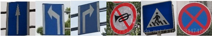
数据集都是我的一个学妹帮忙采集的。在此表示感谢。本文一共选用了6种交通标志,分别为:
数据预处理
一共拍了1465张照片,由于是用手机在路上拍的,图像像素过大且大小不一(有的是横着拍的,有的数竖着拍的),影响检测效率。因此,我先将所有的图片进行了预处理,具体处理步骤为:
(1)以图片宽和高较小的值为裁剪的边长S,从原图中裁剪出S×S的正方形中心区域;
(2)将裁剪出的区域resize为640×640;
处理的主要函数如下:
def center_crop(img_array, crop_size=-1, resize=-1, write_path=None):
    """ crop and resize a square image from the centeral area.
    Args:
        img_array: image array
        crop_size: crop_size (default: -1, min(height, width)).
        resize: resized size (default: -1, keep cropped size)
        write_path: write path of the image (default: None, do not write to the disk).
    Return:
        img_crop: copped and resized image.
    """
    rows = img_array.shape[0]
    cols = img_array.shape[1]

    if crop_size==-1 or crop_size>max(rows,cols):
        crop_size = min(rows, cols)
    row_s = max(int((rows-crop_size)/2), 0)
    row_e = min(row_s+crop_size, rows)
    col_s = max(int((cols-crop_size)/2), 0)
    col_e = min(col_s+crop_size, cols)

    img_crop = img_array[row_s:row_e,col_s:col_e,]

    if resize>0:
        img_crop = cv2.resize(img_crop, (resize, resize))

    if write_path is not None:
        cv2.imwrite(write_path, img_crop)
    return img_crop
def crop_img_dir(img_dir,  save_dir, crop_method = "center", rename_pre=-1):
    """ crop and save square images from original images saved in img_dir.
    Args:
        img_dir: image directory.
        save_dir: save directory.
        crop_method: crop method (default: "center").
        rename_pre: prename of all images (default: -1, use primary image name).
    Return: none
    """
    img_names = os.listdir(img_dir)
    img_names = [img_name for img_name in img_names if img_name.split(".")[-1]=="jpg"]
    index = 0
    for img_name in img_names:
        img = cv2.imread(os.path.join(img_dir, img_name))

        rename = img_name if rename_pre==-1 else rename_pre+str(index)+".jpg"
        img_out_path = os.path.join(save_dir, rename)

        if crop_method == "center":
            img_crop = center_crop(img, resize=640, write_path=img_out_path)

        if index%100 == 0:
            print "total images number = ", len(img_names), "current image number = ", index
        index += 1
数据标注
标注信息采用和PASCAL VOC数据集一样的方式,对于正样本,直接使用labelImg工具进行标注,这里给出我用的一个版本的链接:https://pan.baidu.com/s/1Q0cqJI9Dnvxkj7159Be4Sw。对于负样本,可以使用python中的xml模块自己写xml标注文件,主要函数如下:
from xml.dom.minidom import Document
import os
import cv2

def write_img_to_xml(imgfile, xmlfile):
    """
    write xml file.
    Args:
        imgfile: image file.
        xmlfile: output xml file.
    """
    img = cv2.imread(imgfile)
    img_folder, img_name = os.path.split(imgfile)
    img_height, img_width, img_depth = img.shape
    doc = Document()

    annotation = doc.createElement("annotation")
    doc.appendChild(annotation)

    folder = doc.createElement("folder")
    folder.appendChild(doc.createTextNode(img_folder))
    annotation.appendChild(folder)

    filename = doc.createElement("filename")
    filename.appendChild(doc.createTextNode(img_name))
    annotation.appendChild(filename)

    size = doc.createElement("size")
    annotation.appendChild(size)

    width = doc.createElement("width")
    width.appendChild(doc.createTextNode(str(img_width)))
    size.appendChild(width)

    height = doc.createElement("height")
    height.appendChild(doc.createTextNode(str(img_height)))
    size.appendChild(height)

    depth = doc.createElement("depth")
    depth.appendChild(doc.createTextNode(str(img_depth)))
    size.appendChild(depth)

    with open(xmlfile, "w") as f:
        doc.writexml(f, indent="\t", addindent="\t", newl="\n", encoding="utf-8")
def write_imgs_to_xmls(imgdir, xmldir):
    img_names = os.listdir(imgdir)
    for img_name in img_names:
        img_file = os.path.join(imgdir,img_name)
        xml_file = os.path.join(xmldir, img_name.split(".")[0]+".xml")
        print img_name, "has been written to xml file in ", xml_file
        write_img_to_xml(img_file, xml_file)
数据集划分
这里我们将1465张图片按照7:2:1的比例随机划分为训练集、测试集和验证集。为了方便运行,我们先建立一个名为images的文件夹,下面有JPEGImages和Annotations分别存放了所有的图片和对应的标注文件。同样,最后附上划分数据集的主要函数:
import os
import shutil
import random

def _copy_file(src_file, dst_file):
    """copy file.
    """
    if not os.path.isfile(src_file):
        print"%s not exist!" %(src_file)
    else:
        fpath, fname = os.path.split(dst_file)
        if not os.path.exists(fpath):
            os.makedirs(fpath)
        shutil.copyfile(src_file, dst_file)
def split_data(data_dir, train_dir, test_dir, valid_dir, ratio=[0.7, 0.2, 0.1], shuffle=True):
    """ split data to train data, test data, valid data.
    Args:
        data_dir -- data dir to to be splitted.
        train_dir, test_dir, valid_dir -- splitted dir.
        ratio -- [train_ratio, test_ratio, valid_ratio].
        shuffle -- shuffle or not.
    """
    all_img_dir = os.path.join(data_dir, "JPEGImages/")
    all_xml_dir = os.path.join(data_dir, "Annotations/")
    train_img_dir = os.path.join(train_dir, "JPEGImages/")
    train_xml_dir = os.path.join(train_dir, "Annotations/")
    test_img_dir = os.path.join(test_dir, "JPEGImages/")
    test_xml_dir = os.path.join(test_dir, "Annotations/")
    valid_img_dir = os.path.join(valid_dir, "JPEGImages/")
    valid_xml_dir = os.path.join(valid_dir, "Annotations/")

    all_imgs_name = os.listdir(all_img_dir)
    img_num = len(all_imgs_name)
    train_num = int(1.0*img_num*ratio[0]/sum(ratio))
    test_num = int(1.0*img_num*ratio[1]/sum(ratio))
    valid_num = img_num-train_num-test_num

    if shuffle:
        random.shuffle(all_imgs_name)
    train_imgs_name = all_imgs_name[:train_num]
    test_imgs_name = all_imgs_name[train_num:train_num+test_num]
    valid_imgs_name = all_imgs_name[-valid_num:]

    for img_name in train_imgs_name:
        img_srcfile = os.path.join(all_img_dir, img_name)
        xml_srcfile = os.path.join(all_xml_dir, img_name.split(".")[0]+".xml")
        xml_name = img_name.split(".")[0] + ".xml"

        img_dstfile = os.path.join(train_img_dir, img_name)
        xml_dstfile = os.path.join(train_xml_dir, xml_name)
        _copy_file(img_srcfile, img_dstfile)
        _copy_file(xml_srcfile, xml_dstfile)

    for img_name in test_imgs_name:
        img_srcfile = os.path.join(all_img_dir, img_name)
        xml_srcfile = os.path.join(all_xml_dir, img_name.split(".")[0]+".xml")
        xml_name = img_name.split(".")[0] + ".xml"

        img_dstfile = os.path.join(test_img_dir, img_name)
        xml_dstfile = os.path.join(test_xml_dir, xml_name)
        _copy_file(img_srcfile, img_dstfile)
        _copy_file(xml_srcfile, xml_dstfile)

    for img_name in valid_imgs_name:
        img_srcfile = os.path.join(all_img_dir, img_name)
        xml_srcfile = os.path.join(all_xml_dir, img_name.split(".")[0]+".xml")
        xml_name = img_name.split(".")[0] + ".xml"

        img_dstfile = os.path.join(valid_img_dir, img_name)
        xml_dstfile = os.path.join(valid_xml_dir, xml_name)
        _copy_file(img_srcfile, img_dstfile)
        _copy_file(xml_srcfile, xml_dstfile)
代码运行的结果是在指定的文件夹下分别创建训练集、测试集和验证集文件夹,并且每个文件夹下包含了JPEGImages和Annotations两个子文件夹来存放结果。
到这里用于目标检测的数据集已经准备好了。下面我们介绍整个检测模型的框架。
检测框架
本文用的检测思路非常直观,总的来讲分为候选区域提取、HOG特征提取和SVM分类。
候选区域提取
理论上可以通过设置不同的滑动窗口对整张图像进行遍历,但是这样做不仅计算太大,而且窗口的大小也不好把握。考虑到我们要检测的交通标志都有比较规则的几何形状和颜色信息,我们可以通过检测形状(平行四边形、椭圆)和颜色(红色、蓝色等)来实现初步的预处理以减少计算量,提高检测效率。这里我们以仅颜色信息为例介绍。
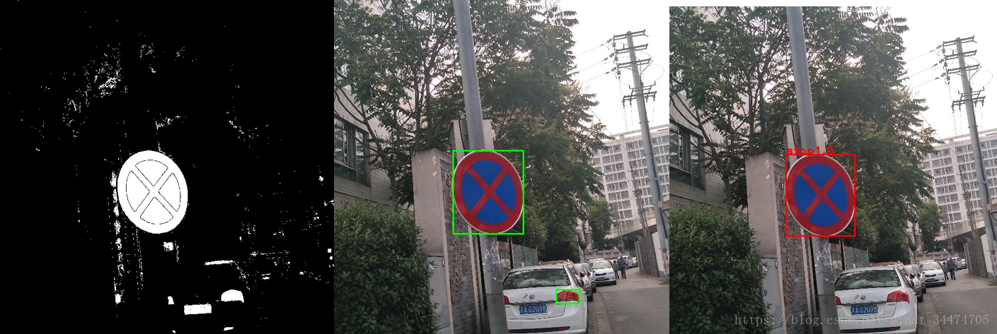
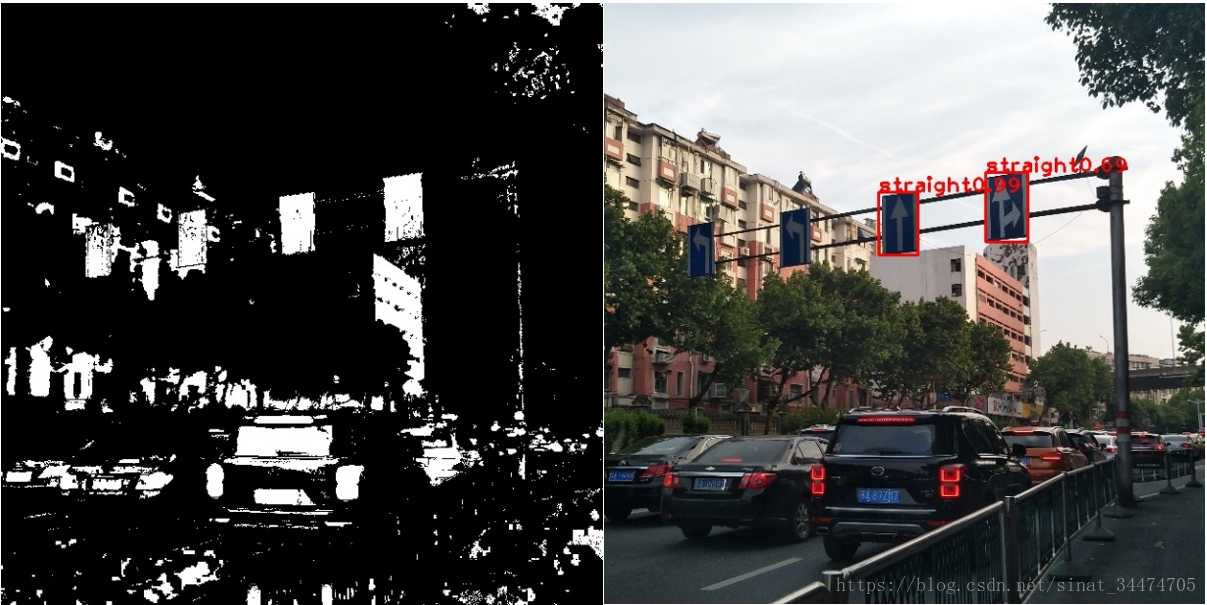
由于需要检测的6类标志主要是红色和蓝色(或者红蓝结合),环境中的不同光照强度可能会使颜色变化较大因此给定一张图像,先在HSV空间中通过颜色阈值分割选出蓝色和红色对应的区域得到二值化图像。然后对二值化图像进行凸包检测(可通过OpenCV实现),下图给出了一个示例:
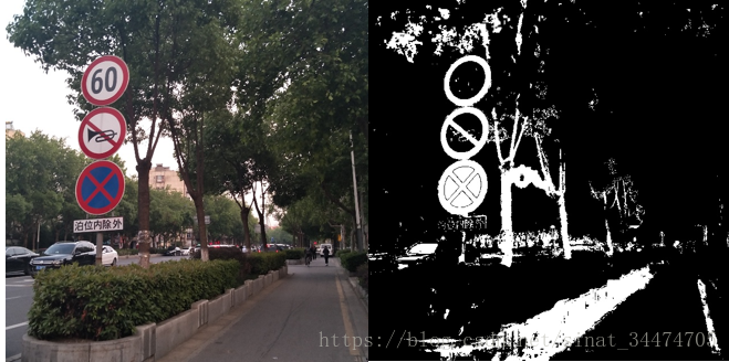
可以看出,经过二值化处理后,图像中的3个标志(其中2个标志是我们需要检测识别的)的轮廓信息都被保留下来了。但是存在依然存在一些问题:(1)背景噪声较多,这会导致检测更多的凸包,从而影响检测速度和精度;(2)三个标志离得很近,可能会导致只检测出一个凸包。我之前考虑过用腐蚀膨胀来滤除一部分的噪声,但在实验的时候发现这会导致更多的漏检。这是因为在腐蚀膨胀的时候部分标志的轮廓信息很有可能会被破坏(尤其是禁止鸣笛标志),导致在凸包检测的阶段被遗漏。所以在最终测试的时候并没有使用腐蚀膨胀操作。下面给出阈值化处理和凸包检测的函数:
def preprocess_img(imgBGR, erode_dilate=True):
    """preprocess the image for contour detection.
    Args:
        imgBGR: source image.
        erode_dilate: erode and dilate or not.
    Return:
        img_bin: a binary image (blue and red).

    """
    rows, cols, _ = imgBGR.shape
    imgHSV = cv2.cvtColor(imgBGR, cv2.COLOR_BGR2HSV)

    Bmin = np.array([100, 43, 46])
    Bmax = np.array([124, 255, 255])
    img_Bbin = cv2.inRange(imgHSV,Bmin, Bmax)

    Rmin1 = np.array([0, 43, 46])
    Rmax1 = np.array([10, 255, 255])
    img_Rbin1 = cv2.inRange(imgHSV,Rmin1, Rmax1)

    Rmin2 = np.array([156, 43, 46])
    Rmax2 = np.array([180, 255, 255])
    img_Rbin2 = cv2.inRange(imgHSV,Rmin2, Rmax2)
    img_Rbin = np.maximum(img_Rbin1, img_Rbin2)
    img_bin = np.maximum(img_Bbin, img_Rbin)

    if erode_dilate is True:
        kernelErosion = np.ones((3,3), np.uint8)
        kernelDilation = np.ones((3,3), np.uint8)
        img_bin = cv2.erode(img_bin, kernelErosion, iterations=2)
        img_bin = cv2.dilate(img_bin, kernelDilation, iterations=2)

    return img_bin
def contour_detect(img_bin, min_area=0, max_area=-1, wh_ratio=2.0):
    """detect contours in a binary image.
    Args:
        img_bin: a binary image.
        min_area: the minimum area of the contours detected.
            (default: 0)
        max_area: the maximum area of the contours detected.
            (default: -1, no maximum area limitation)
        wh_ratio: the ration between the large edge and short edge.
            (default: 2.0)
    Return:
        rects: a list of rects enclosing the contours. if no contour is detected, rects=[]
    """
    rects = []
    _, contours, _ = cv2.findContours(img_bin.copy(), cv2.RETR_EXTERNAL, cv2.CHAIN_APPROX_NONE)
    if len(contours) == 0:
        return rects

    max_area = img_bin.shape[0]*img_bin.shape[1] if max_area<0 else max_area
    for contour in contours:
        area = cv2.contourArea(contour)
        if area >= min_area and area <= max_area:
            x, y, w, h = cv2.boundingRect(contour)
            if 1.0*w/h < wh_ratio and 1.0*h/w < wh_ratio:
                rects.append([x,y,w,h])
    return rects
从函数中可以看出,为了提高候选框的质量,在函数中加入了对凸包面积和外接矩形框长宽比的限制。但需要注意到,凸包的最小面积设置不能太大,否则会导致图片中一些较小的交通标志被漏检。另外,长宽比的限制也不能太苛刻,因为考虑到实际图像中视角的不同,标志的外接矩形框的长宽比可能会比较大。在代码中我的最大长宽比限制为2.5。
这样候选区域虽然选出来了,但是还需要考虑到一件事,我们找出的候选框大小不一,而我们后面的SVM需要固定长度的特征向量,因此在HOG特征提取之前,应把所有的候选区域调整到固定大小(代码中我用的是64×64),这里提供两种解决方案:(1)不管三七二十一,直接将候选区域resize成指定大小,这样做很简单,但是扭曲了原始候选区域的目标信息,不利于SVM的识别(当然,如果用卷积神经网络,这一点问题不是太大,因为卷积神经网络对于物体的扭曲形变有很好的学习能力);(2)提取正方形候选区域,然后resize到指定大小。即对于一个(H×W)的候选框,假设H<W,我们先以长边W围绕候选框中心裁剪出正方形区域,然后再resize,这样做的好处是避免了大部分候选框中目标的扭曲变形。为什么说大部分呢?当某一个候选框在靠近图像边界的时候,如果使用长边裁剪,会出现越界的问题。对于这种情况,我的做法是先沿着边界裁剪出一个矩形区域,再进一步resize成指定大小(细节和代码我会在下面SVM数据集制作上详细介绍)。
HOG特征提取
HOG特征即梯度方向直方图。这里不多介绍,详细的原理可以看我的这篇博客:梯度方向直方图Histogram of Oriented Gradients (HOG)。在具体的实现上是利用skimage库中的feature模块,函数如下:
def hog_feature(img_array, resize=(64,64)):
    """extract hog feature from an image.
    Args:
        img_array: an image array.
        resize: size of the image for extracture.
    Return:
    features:  a ndarray vector.
    """
    img = cv2.cvtColor(img_array, cv2.COLOR_BGR2GRAY)
    img = cv2.resize(img, resize)
    bins = 9
    cell_size = (8, 8)
    cpb = (2, 2)
    norm = "L2"
    features = ft.hog(img, orientations=bins, pixels_per_cell=cell_size,
                        cells_per_block=cpb, block_norm=norm, transform_sqrt=True)
    return features
def extra_hog_features_dir(img_dir, write_txt, resize=(64,64)):
    """extract hog features from images in a directory.
    Args:
        img_dir: image directory.
        write_txt: the path of a txt file used for saving the hog features of all images.
        resize: size of the image for extracture.
    Return:
        none.
    """
    img_names = os.listdir(img_dir)
    img_names = [os.path.join(img_dir, img_name) for img_name in img_names]
    if os.path.exists(write_txt):
        os.remove(write_txt)

    with open(write_txt, "a") as f:
        index = 0
        for img_name in img_names:
            img_array = cv2.imread(img_name)
            features = hog_feature(img_array, resize)
            label_name = img_name.split("/")[-1].split("_")[0]
            label_num = img_label[label_name]

            row_data = img_name + "\t" + str(label_num) + "\t"

            for element in features:
                row_data = row_data + str(round(element,3)) + " "
            row_data = row_data + "\n"
            f.write(row_data)

            if index%100 == 0:
                print "total image number = ", len(img_names), "current image number = ", index
            index += 1
HOG特征提取的一些参数设置可以在函数中看到,如图像尺寸为64×64,设置了9个梯度方向(bin=9)进行梯度信息统计,cell的大小为8×8,每个block包含4个cell(cpb=(2, 2)),标准化方法采用L2标准化(norm=“L2”)。
SVM分类器
对于支持向量机的介绍,网上有一份非常不错的教程:支持向量机通俗导论(理解SVM的三层境界),建议去看一看。我们这里主要是用SVM来对找到的候选区域上提取到的HOG特征做分类。这里我将分别SVM分类器的数据集创建和扩充、模型训练和测试。
数据集创建
这里的数据集和刚开始我们介绍的用于目标检测的数据集不同,我们这边需要构建一个用于分类的数据集。因为已经有了上面的数据,我们可以直接从我们的检测数据中生成。这边我采用的方法和上面介绍的候选区域提取很相似。总体的思路是从目标检测的数据集中裁剪出目标区域作为SVM分类的正样本,同时裁剪出其他的区域(不包含目标的区域)作为负样本。具体的做法如下:
(1)对于包含目标的图片,直接根据标签信息裁剪出一个正方形区域(以长边为边长,少数边界情况需要变形),并移除一些不好的样本(size很小的区域)。这里裁剪出的正样本或多或少包含一部分背景信息,这有利于提高模型对噪声的鲁棒性,同时也为样本较少的情况下数据扩充(如仿射变换)提供了可能。
(2)对于不包含任何目标的图片,通过颜色阈值分割(红色和蓝色)和凸包检测提取一些区域,并裁剪正方形区域(以长边为边长),移除面积较小的区域。与直接随机裁剪相比,这种做法更有针对性,因为在检测提取候选框的时候,很多和交通标志颜色很像的区域会被找出来,直接把这些样本当作负样本对于我们的模型训练很有帮助。
以下是我用的创建正负样本的函数:
解析图片标注信息
def parse_xml(xml_file):
    """parse xml_file
    Args:
        xml_file: the input xml file path
    Returns:
        image_path: string
        labels: list of [xmin, ymin, xmax, ymax, class]
    """
    tree = ET.parse(xml_file)
    root = tree.getroot()
    image_path = ''
    labels = []

    for item in root:
        if item.tag == 'filename':
            image_path = os.path.join(DATA_PATH, "JPEGImages/", item.text)
        elif item.tag == 'object':
            obj_name = item[0].text
            obj_num = classes_num[obj_name]
            xmin = int(item[4][0].text)
            ymin = int(item[4][1].text)
            xmax = int(item[4][2].text)
            ymax = int(item[4][3].text)
            labels.append([xmin, ymin, xmax, ymax, obj_num])
    return image_path, labels
正样本和负样本提取
def produce_pos_proposals(img_path, write_dir, labels, min_size, square=False, proposal_num=0, ):
    """produce positive proposals based on labels.
    Args:
        img_path: image path.
        write_dir: write directory.
        min_size: the minimum size of the proposals.
        labels: a list of bounding boxes.
            [[x1, y1, x2, y2, cls_num], [x1, y1, x2, y2, cls_num], ...]
        square:  crop a square or not.
    Return:
        proposal_num: proposal numbers.
    """
    img = cv2.imread(img_path)
    rows = img.shape[0]
    cols = img.shape[1]
    for label in labels:
        xmin, ymin, xmax, ymax, cls_num = np.int32(label)
        # remove the proposal with small area
        if xmax-xmin<min_size or ymax-ymin<min_size:
            continue
        # crop a square area
        if square is True:
            xcenter = int((xmin + xmax)/2)
            ycenter = int((ymin + ymax)/2)
            size = max(xmax-xmin, ymax-ymin)
            xmin = max(xcenter-size/2, 0)
            xmax = min(xcenter+size/2,cols)
            ymin = max(ycenter-size/2, 0)
            ymax = min(ycenter+size/2,rows)
            proposal = img[ymin:ymax, xmin:xmax]
            proposal = cv2.resize(proposal, (size,size))
        else:
            proposal = img[ymin:ymax, xmin:xmax]

        cls_name = classes_name[cls_num]
        proposal_num[cls_name] +=1
        write_name = cls_name + "_" + str(proposal_num[cls_name]) + ".jpg"
        cv2.imwrite(os.path.join(write_dir,write_name), proposal)
    return proposal_num
def produce_neg_proposals(img_path, write_dir, min_size, square=False, proposal_num=0):
    """produce negative proposals from a negative image.
    Args:
        img_path: image path.
        write_dir: write directory.
        min_size: the minimum size of the proposals.
        square:  crop a square or not.
        proposal_num: current negative proposal numbers.
    Return:
        proposal_num: negative proposal numbers.
    """
    img = cv2.imread(img_path)
    rows = img.shape[0]
    cols = img.shape[1]
    imgHSV = cv2.cvtColor(img, cv2.COLOR_BGR2HSV)
    imgBinBlue = cv2.inRange(imgHSV,np.array([100,43,46]), np.array([124,255,255]))
    imgBinRed1 = cv2.inRange(imgHSV,np.array([0,43,46]), np.array([10,255,255]))
    imgBinRed2 = cv2.inRange(imgHSV,np.array([156,43,46]), np.array([180,255,255]))
    imgBinRed = np.maximum(imgBinRed1, imgBinRed2)
    imgBin = np.maximum(imgBinRed, imgBinBlue)

    _, contours, _ = cv2.findContours(imgBin, cv2.RETR_EXTERNAL, cv2.CHAIN_APPROX_NONE)
    for contour in contours:
        x,y,w,h = cv2.boundingRect(contour)
        if w<min_size or h<min_size:
            continue

        if square is True:
            xcenter = int(x+w/2)
            ycenter = int(y+h/2)
            size = max(w,h)
            xmin = max(xcenter-size/2, 0)
            xmax = min(xcenter+size/2,cols)
            ymin = max(ycenter-size/2, 0)
            ymax = min(ycenter+size/2,rows)
            proposal = img[ymin:ymax, xmin:xmax]
            proposal = cv2.resize(proposal, (size,size))

        else:
            proposal = img[y:y+h, x:x+w]
        write_name = "background" + "_" + str(proposal_num) + ".jpg"
        proposal_num += 1
        cv2.imwrite(os.path.join(write_dir,write_name), proposal)
    return proposal_num
def produce_proposals(xml_dir, write_dir, square=False, min_size=30):
    """produce proposals (positive examples for classification) to disk.
    Args:
        xml_dir: image xml file directory.
        write_dir: write directory of all proposals.
        square: crop a square or not.
        min_size: the minimum size of the proposals.
    Returns:
        proposal_num: a dict of proposal numbers.
    """

    proposal_num = {}
    for cls_name in classes_name:
        proposal_num[cls_name] = 0

    index = 0
    for xml_file in os.listdir(xml_dir):
        img_path, labels = parse_xml(os.path.join(xml_dir,xml_file))
        img = cv2.imread(img_path)
        rows = img.shape[0]
        cols = img.shape[1]

        if len(labels) == 0:
            neg_proposal_num = produce_neg_proposals(img_path, write_dir, min_size, square, proposal_num["background"])
            proposal_num["background"] = neg_proposal_num
        else:
            proposal_num = produce_pos_proposals(img_path, write_dir, labels, min_size, square=True, proposal_num=proposal_num)

        if index%100 == 0:
            print "total xml file number = ", len(os.listdir(xml_dir)), "current xml file number = ", index
            print "proposal num = ", proposal_num
        index += 1

    return proposal_num
上面的返回值proposal_num是用来统计提取的样本数量的。最终我在训练集中获取到的样本数量如下:
proposal_num = {'right': 117, 'straight': 334, 'stop': 224, 'no hook': 168, 'crosswalk': 128, 'left': 208, 'background': 1116}
- 1
裁剪的部分正负样本如下:
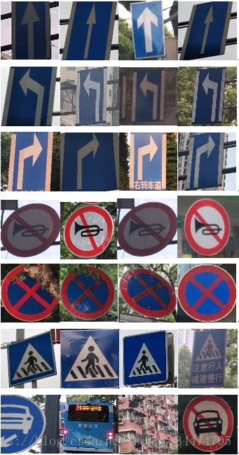
前面几行对应6类正样本,最后一行是背景,可以发现,代码中找出来的背景主要是和我们交通标志颜色(蓝色和红色)相似的区域。我们用相同的方法从我们的验证集中提取正负样本用于SVM模型参数的调整和评估。这里就不再赘述。
训练数据扩充
从上面各个类别样本数量上来看,正样本的各类标志数量相对背景(负样本)很少。为了近些年数据的平衡,我们对正样本进行了扩充。由于我们的数据中包含了向左向右等标志,如何通过旋转或者镜像变换会出问题(当然可以旋转小范围旋转),我也考虑过亮度变换,但是由于HOG特征中引入了归一化方法使得HOG特征对光照不敏感。最终我选用的是仿射变换,这个可以通过OpenCV很方便地实现,具体的仿射变换理论和代码示例可以参考OpenCV官方教程中的Affine Transformations ,这里也给出我对数据集仿射变换的函数:
def affine(img, delta_pix):
    """affine transformation
    Args:
        img: a numpy image array.
        delta_pix: the offset for affine.
    Return:
        res: affined image.
    """
    rows, cols, _ = img.shape
    pts1 = np.float32([[0,0], [rows,0], [0, cols]])
    pts2 = pts1 + delta_pix
    M = cv2.getAffineTransform(pts1, pts2)
    res = cv2.warpAffine(img, M, (rows, cols))
    return res


def affine_dir(img_dir, write_dir, max_delta_pix):
    """ affine transformation on the images in a directory.
    Args:
        img_dir: image directory.
        write_dir: save directory of affined images.
        max_delta_pix: the maximum offset for affine.
    """
    img_names = os.listdir(img_dir)
    img_names = [img_name for img_name in img_names if img_name.split(".")[-1]=="jpg"]
    for index, img_name in enumerate(img_names):
        img = cv2.imread(os.path.join(img_dir,img_name))
        save_name = os.path.join(write_dir, img_name.split(".")[0]+"f.jpg")
        delta_pix = np.float32(np.random.randint(-max_delta_pix, max_delta_pix+1, [3,2]))
        img_a = affine(img, delta_pix)
        cv2.imwrite(save_name, img_a)
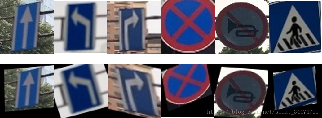
上面函数输入参数max_delta_pix用来控制随机仿射变换的最大强度(正整数),max_delta_pix的绝对值越大,变换越明显(太大可能导致目标信息的完全丢失),我在扩充时这个参数取为10。需要注意的是,10只是变换的最大强度,在对每一张图片进行变换前,会在[-max_delta, max_delta]生成一个随机整数delta_pix(当然你也可以多取几次不同的值来生成更多的变换图片),这个整数控制了当前图片变换的强度。以下是一些变换的结果示例:
模型训练和测试
模型的训练我是直接调用sklearn中的svm库,很多参数都使用了默认值,在训练时发现,惩罚因子C的取值对训练的影响很大,我这边就偷个懒,大概设置了一个值。(超参数可以利用之前的验证集去调整,这里就不赘述了。)用到的函数如下:
def load_hog_data(hog_txt):
    """ load hog features.
    Args:
        hog_txt: a txt file used to save hog features.
            one line data is formated as "img_path \t cls_num \t hog_feature_vector"
    Return:
        img_names: a list of image names.
        labels: numpy array labels (1-dim).
        hog_feature: numpy array hog features.
            formated as [[hog1], [hog2], ...]
    """
    img_names = []
    labels = []
    hog_features = []
    with open(hog_txt, "r") as f:
        data = f.readlines()
        for row_data in data:
            row_data = row_data.rstrip()
            img_path, label, hog_str = row_data.split("\t")
            img_name = img_path.split("/")[-1]
            hog_feature = hog_str.split(" ")
            hog_feature = [float(hog) for hog in hog_feature]
            #print "hog feature length = ", len(hog_feature)
            img_names.append(img_name)
            labels.append(int(label))
            hog_features.append(hog_feature)
    return img_names, np.array(labels), np.array(hog_features)


def svm_train(hog_features, labels, save_path="./svm_model.pkl"):
    """ SVM train
    Args:
        hog_feature: numpy array hog features.
            formated as [[hog1], [hog2], ...]
        labels: numpy array labels (1-dim).
        save_path: model save path.
    Return:
        none.
    """
    clf = SVC(C=10, tol=1e-3, probability = True)
    clf.fit(hog_features, labels)
    joblib.dump(clf, save_path)
    print "finished."

def svm_test(svm_model, hog_feature, labels):
    """SVM test
    Args:
        hog_feature: numpy array hog features.
            formated as [[hog1], [hog2], ...]
        labels: numpy array labels (1-dim).
    Return:
        accuracy: test accuracy.
    """
    clf = joblib.load(svm_model)
    accuracy = clf.score(hog_feature, labels)
    return accuracy
最后,我在3474张训练集(正样本扩充为原来的2倍,负样本没有扩充)上训练,在C=10的时候(其他参数默认),在验证集上(322张)的准确率为97.2%。也就是说有9张图片分类错误,还是可以接受的。
检测结果
回顾一下,我们现在已经可以提取候选区域提取并分类了,也就是说,已经可以对一张完整的图片进行检测了。这里给出我的检测代码和检测结果示例。
import os
import numpy as np
import cv2
from skimage import feature as ft
from sklearn.externals import joblib

cls_names = ["straight", "left", "right", "stop", "nohonk", "crosswalk", "background"]
img_label = {"straight": 0, "left": 1, "right": 2, "stop": 3, "nohonk": 4, "crosswalk": 5, "background": 6}

def preprocess_img(imgBGR, erode_dilate=True):
    """preprocess the image for contour detection.
    Args:
        imgBGR: source image.
        erode_dilate: erode and dilate or not.
    Return:
        img_bin: a binary image (blue and red).

    """
    rows, cols, _ = imgBGR.shape
    imgHSV = cv2.cvtColor(imgBGR, cv2.COLOR_BGR2HSV)

    Bmin = np.array([100, 43, 46])
    Bmax = np.array([124, 255, 255])
    img_Bbin = cv2.inRange(imgHSV,Bmin, Bmax)

    Rmin1 = np.array([0, 43, 46])
    Rmax1 = np.array([10, 255, 255])
    img_Rbin1 = cv2.inRange(imgHSV,Rmin1, Rmax1)

    Rmin2 = np.array([156, 43, 46])
    Rmax2 = np.array([180, 255, 255])
    img_Rbin2 = cv2.inRange(imgHSV,Rmin2, Rmax2)
    img_Rbin = np.maximum(img_Rbin1, img_Rbin2)
    img_bin = np.maximum(img_Bbin, img_Rbin)

    if erode_dilate is True:
        kernelErosion = np.ones((9,9), np.uint8)
        kernelDilation = np.ones((9,9), np.uint8)
        img_bin = cv2.erode(img_bin, kernelErosion, iterations=2)
        img_bin = cv2.dilate(img_bin, kernelDilation, iterations=2)

    return img_bin


def contour_detect(img_bin, min_area=0, max_area=-1, wh_ratio=2.0):
    """detect contours in a binary image.
    Args:
        img_bin: a binary image.
        min_area: the minimum area of the contours detected.
            (default: 0)
        max_area: the maximum area of the contours detected.
            (default: -1, no maximum area limitation)
        wh_ratio: the ration between the large edge and short edge.
            (default: 2.0)
    Return:
        rects: a list of rects enclosing the contours. if no contour is detected, rects=[]
    """
    rects = []
    _, contours, _ = cv2.findContours(img_bin.copy(), cv2.RETR_EXTERNAL, cv2.CHAIN_APPROX_NONE)
    if len(contours) == 0:
        return rects

    max_area = img_bin.shape[0]*img_bin.shape[1] if max_area<0 else max_area
    for contour in contours:
        area = cv2.contourArea(contour)
        if area >= min_area and area <= max_area:
            x, y, w, h = cv2.boundingRect(contour)
            if 1.0*w/h < wh_ratio and 1.0*h/w < wh_ratio:
                rects.append([x,y,w,h])
    return rects


def draw_rects_on_img(img, rects):
    """ draw rects on an image.
    Args:
        img: an image where the rects are drawn on.
        rects: a list of rects.
    Return:
        img_rects: an image with rects.
    """
    img_copy = img.copy()
    for rect in rects:
        x, y, w, h = rect
        cv2.rectangle(img_copy, (x,y), (x+w,y+h), (0,255,0), 2)
    return img_copy


def hog_extra_and_svm_class(proposal, clf, resize = (64, 64)):
    """classify the region proposal.
    Args:
        proposal: region proposal (numpy array).
        clf: a SVM model.
        resize: resize the region proposal
            (default: (64, 64))
    Return:
        cls_prop: propabality of all classes.
    """
    img = cv2.cvtColor(proposal, cv2.COLOR_BGR2GRAY)
    img = cv2.resize(img, resize)
    bins = 9
    cell_size = (8, 8)
    cpb = (2, 2)
    norm = "L2"
    features = ft.hog(img, orientations=bins, pixels_per_cell=cell_size,
                        cells_per_block=cpb, block_norm=norm, transform_sqrt=True)
    print "feature = ", features.shape
    features = np.reshape(features, (1,-1))
    cls_prop = clf.predict_proba(features)
    print("type = ", cls_prop)
    print "cls prop = ", cls_prop
    return cls_prop


if __name__ == "__main__":
    img = cv2.imread("/home/meringue/Documents/traffic_sign_detection/svm_hog_classification/sign_89.jpg")
    rows, cols, _ = img.shape
    img_bin = preprocess_img(img,False)
    cv2.imshow("bin image", img_bin)
    cv2.imwrite("bin_image.jpg", img_bin)
    min_area = img_bin.shape[0]*img.shape[1]/(25*25)
    rects = contour_detect(img_bin, min_area=min_area)
    img_rects = draw_rects_on_img(img, rects)
    cv2.imshow("image with rects", img_rects)
    cv2.imwrite("image_rects.jpg", img_rects)

    clf = joblib.load("./svm_model.pkl")

    img_bbx = img.copy()

    for rect in rects:
        xc = int(rect[0] + rect[2]/2)
        yc = int(rect[1] + rect[3]/2)

        size = max(rect[2], rect[3])
        x1 = max(0, int(xc-size/2))
        y1 = max(0, int(yc-size/2))
        x2 = min(cols, int(xc+size/2))
        y2 = min(rows, int(yc+size/2))
        proposal = img[y1:y2, x1:x2]
        cls_prop = hog_extra_and_svm_class(proposal, clf)
        cls_prop = np.round(cls_prop, 2)[0]
        cls_num = np.argmax(cls_prop)
        cls_name = cls_names[cls_num]
        prop = cls_prop[cls_num]
        if cls_name is not "background":
            cv2.rectangle(img_bbx,(rect[0],rect[1]), (rect[0]+rect[2],rect[1]+rect[3]), (0,0,255), 2)
            cv2.putText(img_bbx, cls_name+str(prop), (rect[0], rect[1]), 1, 1.5, (0,0,255),2)

    cv2.imshow("detect result", img_bbx)
    cv2.imwrite("detect_result.jpg", img_bbx)
    cv2.waitKey(0)
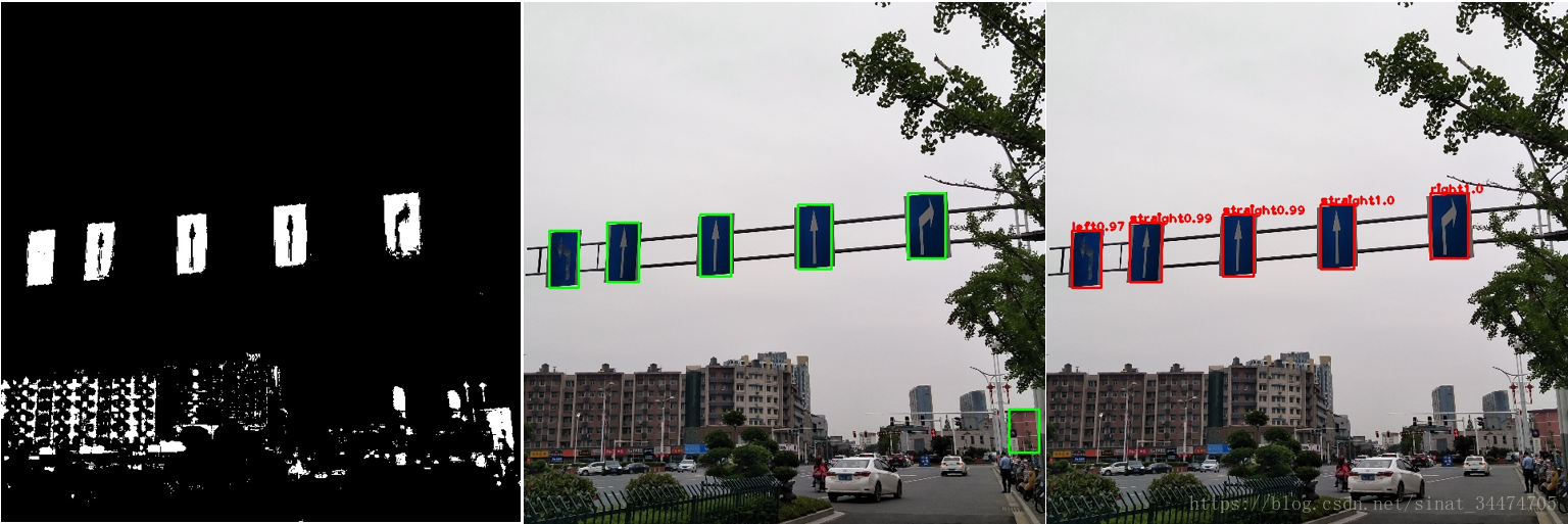
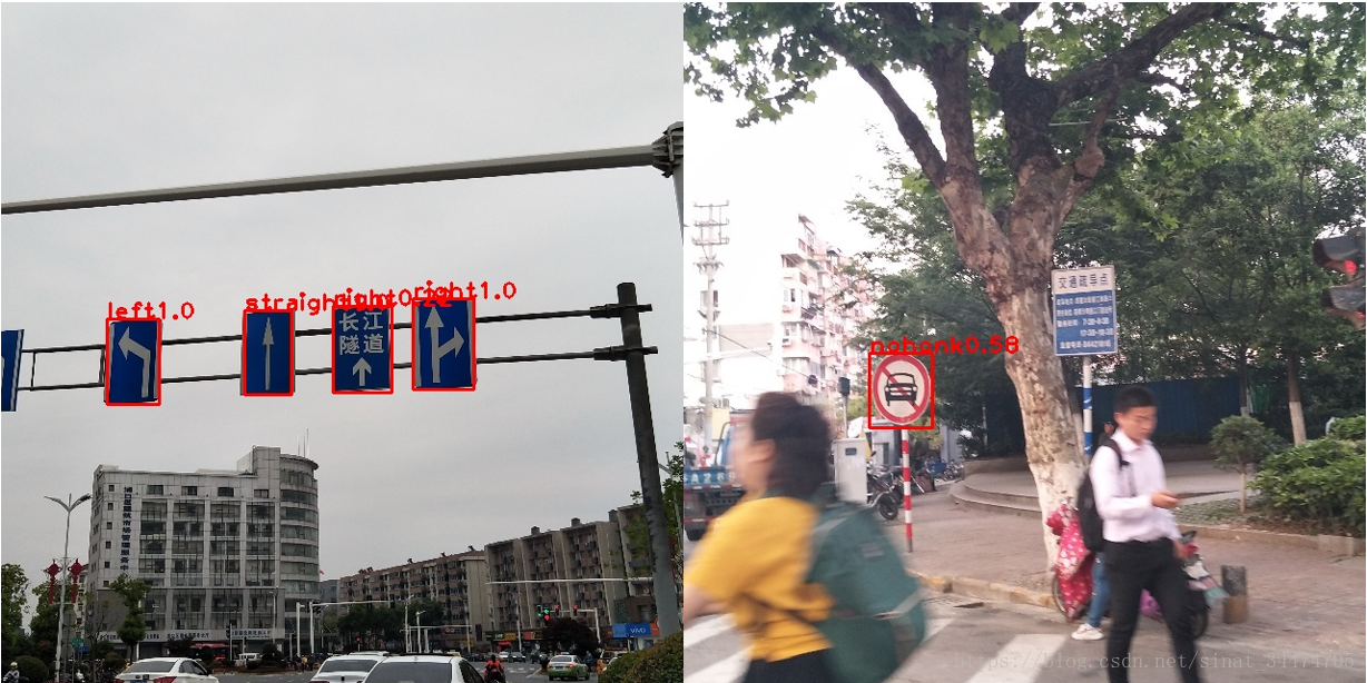
上图中从左到右分别为阈值化后的图、候选框提取结果和最终检测检测结果(类别名+置信度),最终各个类别标志的准确率和召回率(IOU的阈值设为0.5)如下(计算的代码在我的github里可以找到,就不放在博客里了。):
| 标志 | 直行 | 左转 | 右转 | 禁止鸣笛 | 人行横道 | 禁止通行 |
|---|---|---|---|---|---|---|
| 准确率 | 41.6% | 45.8% | 43.5% | 45.3% | 75.6% | 45.7% |
| 召回率 | 37.1% | 39.8% | 43.5% | 48.3% | 50.8% | 57.1% |
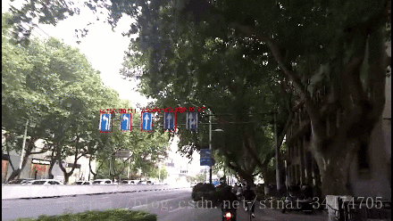
用于视频中的实时检测视频示例:
对SVM输出的概率值依次设置0.1、0.2 …0.9的阈值,得到的平均准确率和召回率变化趋势如下:
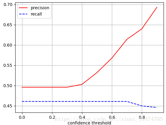
从数据上可以发现,总体的检测结果还是很不理想的。我们通过观察准确率和召回率的变化曲线发现,当置信度的阈值不断变大时,平均准确率不断上升,而召回率比较平缓(阈值大于0.7的时候略微下降)。进一步观察检测的图片发现,候选区域的提取是我们检测模型性能的瓶颈,这主要体现在以下两点:
(1)有很多标志所在的候选区域被漏检(详见Bad Cases Analysis),这直接导致最终的召回率很低。
(2)有些包含标志的候选区域虽然被找出来了,但是其中包含了大量的噪声,如出现相似颜色的背景时,标志只占候选区域的一小部分,或者多个标志相邻时被框在了一起,这将直接影响分类的结果,降低准确率。
而提高置信度时,大量的误检会被排除,而漏检情况几乎不受影响(候选区域的提取不受置信度阈值的影响),所以会明显提高准确率。
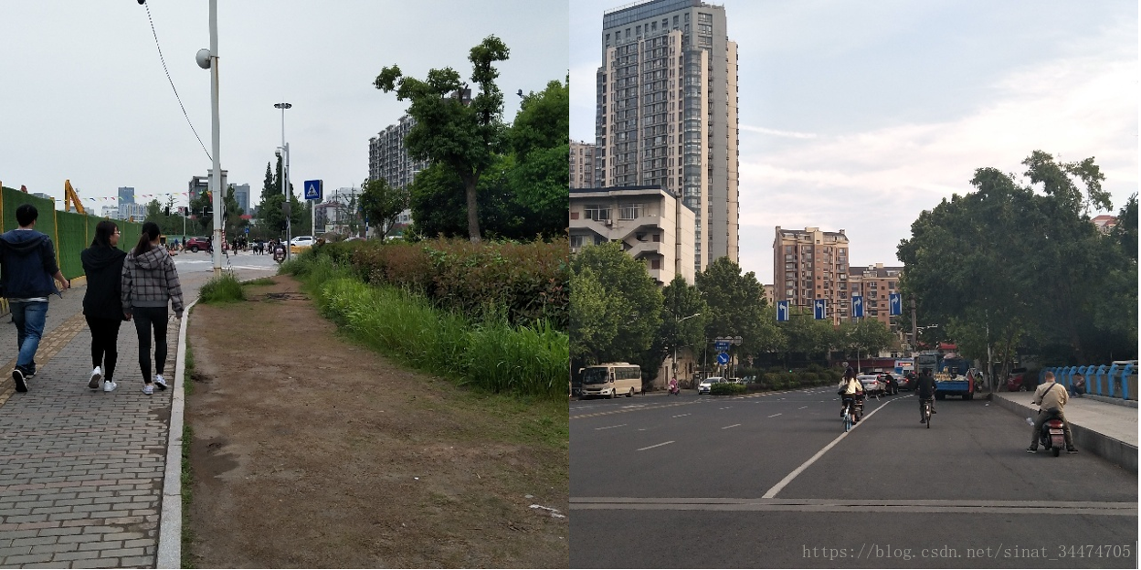
Bad Cases Analysis
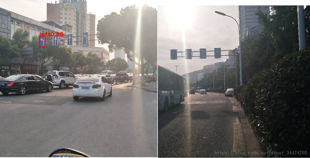
基于上面的检测结果,我把所有的检测矩形框在图像中画出来,并一一查看,发现误检和漏检问题主要体现在一下几个方面:
**光线不均匀。**由于图片都是在不同的时刻从户外进行采集的,测试集中的部分交通标志存在在强光和弱光的情况,这将直接对候选区域的提取造成困难。虽然我们在颜色空间上已经选用了对光线鲁棒性较好的HSV空间,但仍然无法避免光照过于恶劣的情况。不过我发现,光照对分类的影响很小,这是因为我们使用的HOG特征里有标准化的操作,使得同一个候选框在不同的光照下HOG特征保持不变。我实验的时候考虑过适当放宽蓝色和红色的阈值范围,但是这样做也会产生更多的背景框,影响检测速度。
**复杂或相似的背景干扰。**我们的阈值化是基于颜色信息的,所以当标志物周围有颜色相近的背景时(如楼房、蓝天等),会很大程度上对候选框的提取造成影响。如下图中,由于左边的两个标志周围有颜色接近红色的小区的干扰,所以在阈值化时周围包含了大量的噪声,对SVM的分类影响很大。可以考虑加入轻微的腐蚀膨胀来弱化噪声的影响,但对于一些较小甚至不完全封闭的标志,会破坏原有的结构,造成漏检。
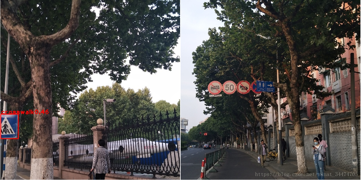
**局部遮挡或缺失。**这两种情况相当于在特征提取过程中加入了噪声,对候选框提取的影响较小,它主要影响分类器的识别。可以在SVM训练集中加入部分包含遮挡的标志来提高鲁棒性。下图中左边虽然还是检测除了人行横道标志,但置信度很低。
多个标志相邻
这种情况在实际场景中非常常见,当多个标志连在一起的时候,凸包检测的过程中会把几个标志当成一个整体,从而导致漏检和误检。
相似标志或背景的干扰
我们在检测的时候只选取了6类标志,所以其他标志都相当于是背景。但是,在检测的时候有些标志和我们的6类标志很像,提高了分类的难度,从而造成误检。
小目标检测
当目标较小的时候,我们在HOG特征提取之前先进行了resize操作,但resize后的图像往往不能准确的反映小目标的HOG特征(分辨率过低),导致提取的特征很粗糙,不利于分类。
改进思路
整个检测框架的瓶颈是候选区域的选取。由于我只使用了颜色信息进行候选框提取,因此存在大量的噪声,很容易导致候选区域提取阶段漏掉部分标志。所以比较有效的一个改进思路是优化候选框的提取过程,比如加入一些形状的检测(平行四边形、椭圆等),但由于形状检测的计算量比较大,可能会降低整体的检测速度。当应用视频中的实时检测时,速度可能会跟不上。
另外,虽然这边SVM的分类效果还可以接受,但这仅仅是7(6+1)个类别,当样本类别很多时,需要更多的数据和更强大的分类器(如卷积神经网络)来降低误检率。
最后再提下一个暴力的改进思路是直接扔掉候选区域提取的过程,改用像YOLO网络这样端到端的检测框架。总之,思路很多,感兴趣的朋友可以自己去尝试。
写在最后的话:
感谢你一直读到这里,希望这篇的博客对你能有点帮助,关于本篇博客中的任何问题欢迎指出,虚心接受各位大佬的教导!